Eaton method with well log
Pore pressure prediction with Eaton’s method using well log data.
Steps:
Calculate Velocity Normal Compaction Trend
Optimize for Eaton’s exponent n
Predict pore pressure using Eaton’s method
[2]:
from __future__ import print_function, division, unicode_literals
%matplotlib inline
import matplotlib.pyplot as plt

plt.style.use(['seaborn-paper', 'seaborn-whitegrid'])
plt.rcParams['font.sans-serif']=['SimHei']
plt.rcParams['axes.unicode_minus']=False

import numpy as np

import pygeopressure as ppp
1. Calculate Velocity Normal Compaction Trend
Create survey with the example survey CUG:
[3]:
# set to the directory on your computer
SURVEY_FOLDER = "C:/Users/yuhao/Desktop/CUG_depth"

survey = ppp.Survey(SURVEY_FOLDER)
Retrieve well CUG1:
[4]:
well_cug1 = survey.wells['CUG1']
Get velocity log:
[5]:
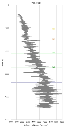
vel_log = well_cug1.get_log("Velocity")
View velocity log:
[6]:
fig_vel, ax_vel = plt.subplots()
ax_vel.invert_yaxis()
vel_log.plot(ax_vel)
well_cug1.plot_horizons(ax_vel)

# set fig style
ax_vel.set(ylim=(5000,0), aspect=(5000/4600)*2)
ax_vel.set_aspect(2)
fig_vel.set_figheight(8)
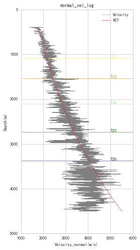
Optimize for NCT coefficients a, b:
well.params['horizon']['T20'] returns the depth of horizon T20.
[7]:
a, b = ppp.optimize_nct(
    vel_log=well_cug1.get_log("Velocity"),
    fit_start=well_cug1.params['horizon']["T16"],
    fit_stop=well_cug1.params['horizon']["T20"])
And use a, b to calculate normal velocity trend
[8]:
from pygeopressure.velocity.extrapolate import normal_log
nct_log = normal_log(vel_log, a=a, b=b)
View fitted NCT:
[9]:
fig_vel, ax_vel = plt.subplots()
ax_vel.invert_yaxis()
# plot velocity
vel_log.plot(ax_vel, label='Velocity')
# plot horizon
well_cug1.plot_horizons(ax_vel)
# plot fitted nct
nct_log.plot(ax_vel, color='r', zorder=2, label='NCT')

# set fig style
ax_vel.set(ylim=(5000,0), aspect=(5000/4600)*2)
ax_vel.set_aspect(2)
ax_vel.legend()
fig_vel.set_figheight(8)
Save fitted nct:
[10]:
# well_cug1.params['nct'] = {"a": a, "b": b}

# well_cug1.save_params()
2. Optimize for Eaton’s exponent n
First, we need to preprocess velocity.
Velocity log processing (filtering and smoothing):
[11]:
vel_log_filter = ppp.upscale_log(vel_log, freq=20)

vel_log_filter_smooth = ppp.smooth_log(vel_log_filter, window=1501)
Veiw processed velocity:
[12]:
fig_vel, ax_vel = plt.subplots()
ax_vel.invert_yaxis()
# plot velocity
vel_log.plot(ax_vel, label='Velocity')
# plot horizon
well_cug1.plot_horizons(ax_vel)
# plot processed velocity
vel_log_filter_smooth.plot(ax_vel, color='g', zorder=2, label='Processed', linewidth=1)

# set fig style
ax_vel.set(ylim=(5000,0), aspect=(5000/4600)*2)
ax_vel.set_aspect(2)
ax_vel.legend()
fig_vel.set_figheight(8)
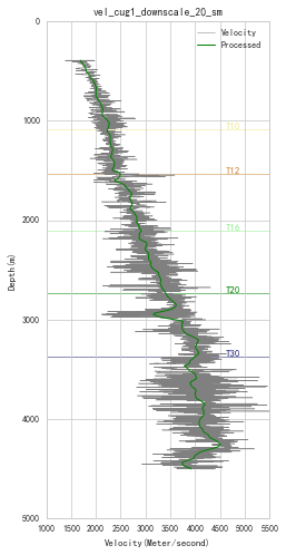
We will use the processed velocity data for pressure prediction.
Optimize Eaton’s exponential n:
[13]:
n = ppp.optimize_eaton(
    well=well_cug1,
    vel_log=vel_log_filter_smooth,
    obp_log="Overburden_Pressure",
    a=a, b=b)
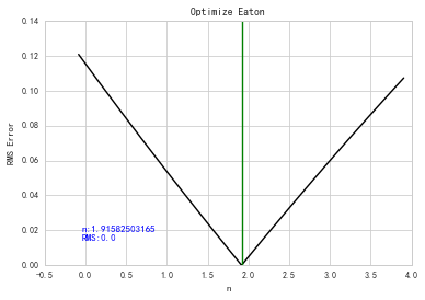
See the RMS error variation with n:
[14]:
from pygeopressure.basic.plots import plot_eaton_error

fig_err, ax_err = plt.subplots()

plot_eaton_error(
    ax=ax_err,
    well=well_cug1,
    vel_log=vel_log_filter_smooth,
    obp_log="Overburden_Pressure",
    a=a, b=b)
Save optimized n:
[15]:
# well_cug1.params['nct'] = {"a": a, "b": b}

# well_cug1.save_params()
3.Predict pore pressure using Eaton’s method
Calculate pore pressure using Eaton’s method requires velocity, Eaton’s exponential, normal velocity, hydrostatic pressure and overburden pressure.
Well.eaton() will try to read saved data, users only need to specify them when they are different from the saved ones.
[16]:
pres_eaton_log = well_cug1.eaton(vel_log_filter_smooth, n=n)
View predicted pressure:
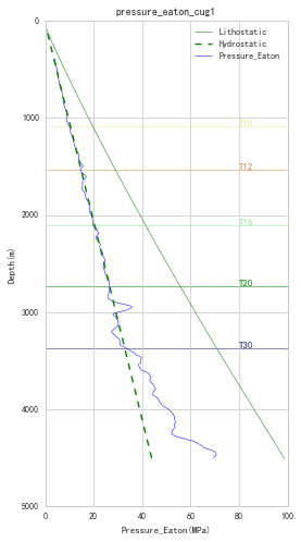
[17]:
fig_pres, ax_pres = plt.subplots()
ax_pres.invert_yaxis()

well_cug1.get_log("Overburden_Pressure").plot(ax_pres, 'g', label='Lithostatic')
ax_pres.plot(well_cug1.hydrostatic, well_cug1.depth, 'g', linestyle='--', label="Hydrostatic")
pres_eaton_log.plot(ax_pres, color='blue', label='Pressure_Eaton')
well_cug1.plot_horizons(ax_pres)

# set figure and axis size
ax_pres.set_aspect(2/50)
ax_pres.legend()
fig_pres.set_figheight(8)