Eaton Method with Seismic Velocity Data

from __future__ import print_function, division, unicode_literals
%matplotlib inline
import matplotlib.pyplot as plt

plt.style.use(['seaborn-paper', 'seaborn-whitegrid'])
plt.rcParams['font.sans-serif']=['SimHei']
plt.rcParams['axes.unicode_minus']=False

import numpy as np

import pygeopressure as ppp

Create survey CUG:

# set to the directory on your computer
SURVEY_FOLDER = "M:/CUG_depth"

survey = ppp.Survey(SURVEY_FOLDER)

Retrieve well CUG1:

well_cug1 = survey.wells['CUG1']

Get a, b from well CUG1:

a = well_cug1.params['nct']["a"]
b = well_cug1.params['nct']["b"]

Get n from well CUG1:

n = well_cug1.params['n']

Retrieve seismic data:

vel_cube = survey.seismics['velocity']
obp_cube = survey.seismics['obp_new']

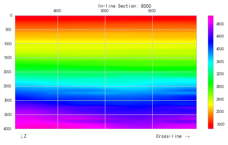
View velocity section:

fig_vel, ax_vel = plt.subplots()

im = vel_cube.plot(
    ppp.InlineIndex(8000), ax_vel, kind='img', cm='gist_rainbow')
fig_vel.colorbar(im)
fig_vel.set(figwidth=8)

[None]

Pressure Prediction with Eaton method:

eaton_cube = ppp.eaton_seis(
    "eaton_new", obp_cube, vel_cube, n=3,
    upper=survey.horizons['T16'], lower=survey.horizons['T20'])

eaton_seis function will automatically optimize the coefficients of Normal Compaction Trend, a and b.

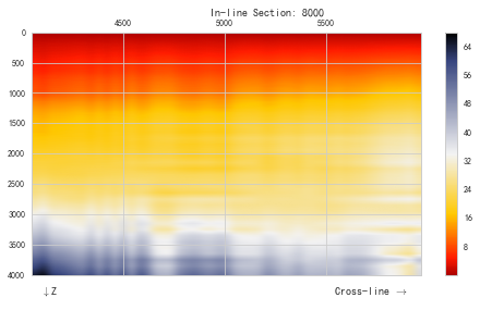
View calculated pressure:

from pygeopressure.basic.vawt import opendtect_seismic_colormap

fig_pres, ax_pres = plt.subplots()

im = eaton_cube.plot(
    ppp.InlineIndex(8000), ax_pres,
    kind='img', cm=opendtect_seismic_colormap())

fig_pres.colorbar(im)
fig_pres.set(figwidth=8)

[None]