Bowers method with well log¶

Pore pressure prediction with Bowers’ method using well log data.

Predicton of geopressure using Bowers’ model needs the following steps:

determine Bowers loading equation coefficients A and B
determine Bowers unloading equation coefficients \(V_{max}\) and U
Pressure Prediction

[2]:

from __future__ import print_function, division, unicode_literals
%matplotlib inline
import matplotlib.pyplot as plt

plt.style.use(['seaborn-paper', 'seaborn-whitegrid'])
plt.rcParams['font.sans-serif']=['SimHei']
plt.rcParams['axes.unicode_minus']=False

import numpy as np

import pygeopressure as ppp

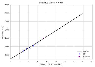
1. determine Bowers loading equation coefficients A and B¶

Create survey with the example survey CUG:

[3]:

# set to the directory on your computer
SURVEY_FOLDER = "M:/CUG_depth"

survey = ppp.Survey(SURVEY_FOLDER)

Retrieve well CUG1:

[4]:

well_cug1 = survey.wells['CUG1']

Get velocity log:

[5]:

vel_log = well_cug1.get_log("Velocity")

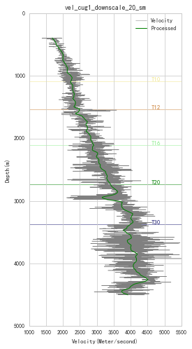
Preprocessing velocity data

[6]:

vel_log_filter = ppp.upscale_log(vel_log, freq=20)

vel_log_filter_smooth = ppp.smooth_log(vel_log_filter, window=1501)

View velocity and processed velocity

[7]:

fig_vel, ax_vel = plt.subplots()
ax_vel.invert_yaxis()
# plot velocity
vel_log.plot(ax_vel, label='Velocity')
# plot horizon
well_cug1.plot_horizons(ax_vel)
# plot processed velocity
vel_log_filter_smooth.plot(ax_vel, color='g', zorder=2, label='Processed', linewidth=1)

# set fig style
ax_vel.set(ylim=(5000,0), aspect=(4600/5000)*2)
ax_vel.legend()
fig_vel.set_figheight(8)

../_images/tutorial_bowers_well_14_0.png

Optimize for Bowers’ loading equation coefficients A, B:

[8]:

a, b, err = ppp.optimize_bowers_virgin(
    well=well_cug1,
    vel_log=vel_log_filter_smooth,
    obp_log='Overburden_Pressure',
    upper='T12',
    lower='T20',
    pres_log='loading',
    mode='both')

Plot optimized virgin curve:

[9]:

fig_bowers, ax_bowers = plt.subplots()

ppp.plot_bowers_vrigin(
    ax=ax_bowers,
    well=well_cug1,
    a=a,
    b=b,
    vel_log=vel_log_filter_smooth,
    obp_log='Overburden_Pressure',
    upper='T12',
    lower='T20',
    pres_log='loading',
    mode='both')

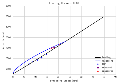
../_images/tutorial_bowers_well_18_0.png

2. determine Bowers unloading equation coefficients \(V_{max}\) and U¶

After manually select paramter U, optimze for parameter U:

[10]:

u = ppp.optimize_bowers_unloading(
    well=well_cug1,
    vel_log=vel_log_filter_smooth,
    obp_log='Overburden_Pressure',
    a=a,
    b=b,
    vmax=4600,
    pres_log='unloading')

Draw unloading curve and virgin curve together with optimized parameters:

[11]:

fig_bowers, ax_bowers = plt.subplots()
# draw virgin(loading) curve
ppp.plot_bowers_vrigin(
    ax=ax_bowers,
    well=well_cug1,
    a=a,
    b=b,
    vel_log=vel_log_filter_smooth,
    obp_log='Overburden_Pressure',
    upper='T12',
    lower='T20',
    pres_log='loading',
    mode='both')

# draw unloading curve
ppp.plot_bowers_unloading(
    ax=ax_bowers,
    a=a,
    b=b,
    vmax=4600,
    u=u,
    well=well_cug1,
    vel_log=vel_log_filter_smooth,
    obp_log='Overburden_Pressure',
    pres_log='unloading')

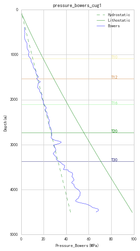
../_images/tutorial_bowers_well_23_0.png

3. Pressure Prediction with Bowers model¶

predict pressure with coefficients calculated above:

[12]:

pres_log = well_cug1.bowers(
    vel_log=vel_log_filter_smooth, a=a, b=b, u=u)

View Bowers Pressure Results:

[13]:

fig_pres, ax_pres = plt.subplots()
ax_pres.invert_yaxis()
# plot hydrostatic
well_cug1.hydro_log().plot(ax_pres, linestyle='--', color='green', label='Hydrostatic')
# plot OBP
well_cug1.get_log("Overburden_Pressure").plot(ax_pres, color='green', label='Lithostatic')
# plot pressure
pres_log.plot(ax_pres, label='Bowers', color='blue')
# plot horizon
well_cug1.plot_horizons(ax_pres)


# set fig style
ax_pres.set(ylim=(5000,0), aspect=(100/5000)*2)
ax_pres.legend()
fig_pres.set_figheight(8)

../_images/tutorial_bowers_well_28_0.png